Measurement and visualization of parallelism

At parallel 2012 (Slides in German) we have shown how to measure and illustrate software parallelism. This article will expand/elaborate by using a simple route planner written in C++11. We'll show how to parallelize an algorithm and how to showcase and verify runtime measurements.

The image on the right shows the 10 largest cities in Germany (Source: Wikipedia) in a map of Germany (Source: Wikipedia). We want to find the shortest path visiting all those cities (straight line distance).

First, we implement a serial (not parallelized) algorithm for this task. Then, we'll use a simple technique - by using OpenMP - for parallelizing this task. We'll then show how to compute the so-called SpeedUp Factor.

Later blog articles will show other techniques for parallelization (by using CilkPlus or by explicit parallelization via C++-11 threads). All of those techniques are available to us by using the g++ compiler (CilkPlus starting with version 4.9.0).

In order to show a practical approach for parallelization we have chose a simple but quite compute-intensive problem:

• Given a set of num (in our case 10) cities in Germany
• ... find a shortest path (straight line distance) starting from the first city and visiting all others

As the number of cities increases the effort required to compute the shortest path also does.

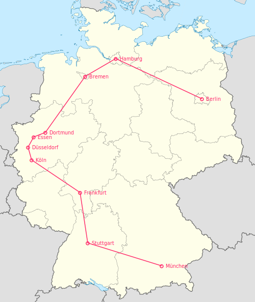
We have drawn the shortest path visiting all cities into the map shown at the right. This path should be our result in the following computations. If, for example, we had chosen Düsseldorf as our starting city, the solution naturally wouldn't be as obvious. But for now our approach to solving the given problem:

As our shortest path could be any permutation of the given cities we have to consider all those paths. In order to find all paths we can do as shown in the following pseudo-code:

Function calcMinRoute(ListOfCities, Route, MinRoute)
  If ListOfCities.Length > 1 Then
    ForEach ListOfCities Do
      Remaining = ListOfCities
      Remaining.Remove(Current)
      Route.PushBack(Current)
      calcMinRoute(Remaining, Route, MinRoute)
      Route.PopBack()
    Done
  Else
    Route.PushBack(ListOfCities[0])
    Distance = CalcDistance(ArrayOfParents);
    Route.PopBack()
    If Distance < MinRoute.Distance Then
      MinRoute.Distance = Distance
      MinRoute.Route = Route
    EndIf
  EndIf
EndFunc

Implementation

CityDB

This class implements reading in (from a database) and management of all cities. We use the OpenGeoDB database of cities for Germany.

City

A simple class that represents exactly one class together with its name, postal code and coordinates

myARM

Simple class encapsulating all information needed for measurements with the Application Response Measurement ARM 4.0 standard

myRoute

The main program for computing the shortest path

ompRoute

The main program for computing the shortest path with OpenMP parallelization

We will not discuss the algorithm in detail in the following sections. Instead we will provide a brief instruction on how to measure the response times with the ARM 4.0 standard and how to use these measurements to compute the SpeedUp factor.

The MyARM ARM 4.0 C++ implementation is loosely based on the ARM 4.0 Java binding. This C++ implementation is built on top of the ARM 4.0 C binding. By means of dynamic loading of the ARM 4.0 library (libarm4.so), an ARM 4.0 C implementation is loaded and thus used. A real ARM 4.0 C++ binding had not been expedited during standardization because of the then-unstable ABI.

In order to be able to correlate measurements with the corresponding code sequences during analysis, ARM 4.0 provides some concepts for the naming of applications (ArmApplicationDefinition) and of measurements (ArmTransactionDefinition). In our example we will use the program's name (argv[0]), thus myRoute for the serial and ompRoute for the parallel version (via OpenMP) as application name and the following names for the measurements (transaction name):

MinRoute

records the response time for the entire computation of the shortest path

ReadCityDB

records the response time for reading in OpenGeoDB data from a file and saving it in c++ containers

CalcRoute

records the response time for the computation of all paths and the ensuing identification of the shortest path

PartialRoutes

records the response time for the computation of a single path

As an example we will now discuss two measurements for the response times of MinRoute and CalcRoute:

1. the entire response time is provided by the measurement named MinRoute. For this purpose we instrument the function main() of the myRoute program:

   using namespace arm4;
   int main(int argc, char *argv[])
   {
      std::string prg = basename(argv[0]);
      ...
      // create all ARM meta and application instances
      myARM::instance = new myARM(prg);
   
      // create and start our main measurement
      ArmTransaction minRoute(myARM::instance->myApp_, myARM::instance->minRouteDef_);
      // start our main measurement
      minRoute.start();
      // remember our main correlator for other sub-measurements
      myARM::instance->mainCorr_ = minRoute.getCorrelator();
      // real work take place here
      ...
      // stop our main measurement with status good
      minRoute.stop(ArmConstants::STATUS_GOOD);
      return 0;
   }
   

2. the response time measurement for the calculation of the shortest path named CalcRoute is done like this:

   void minDistanceRoute(const std::vector<City*>& cities)
   {
      // start the minimal route calculation measurement
      ArmTransaction calcRoute(myARM::instance->myApp_, myARM::instance->calcRoutesDef_);
      // use the correlator of the main measurement as the parent of our measurement
      calcRoutes.start(myARM::instance->mainCorr_);
      // real minimum distance calculation takes place here
      ...
      // stop the minimal route calculation measurement
      calcRoute.stop(ArmConstants::STATUS_GOOD);
   }
   

After having instrumented the application with ARM 4.0 we now compute the shortest path for the 10 largest cities in Germany. We invoke our program like that:

./myRoute Berlin Hamburg München Köln "Frankfurt am Main" Stuttgart Dortmund \
Düsseldorf "Essen, Ruhr" Bremen

We chose the capital Berlin as starting point and thus specify it as first argument in the command. All other cities can be specified in arbitrary order. We get the following result:

number of routes: 362880
route: |-- Berlin --[255.292km]--> Hamburg --[95.2193km]--> Bremen --[196.644km]--> Dortmund --[33.239km]--> Essen, Ruhr --[30.189km]--> Düsseldorf --[33.377km]--> Köln --[152.598km]--> Frankfurt am Main --[152.705km]--> Stuttgart --[190.955km]--> München--| total distance is 1140.22km.

The number of computed paths is displayed first, then the shortest path found, together with the associated distances between each pair of adjacent cities.

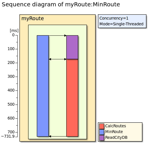
By using the MyARM myarmbrowser application we get the sequence diagram shown on the right side:

As you can see in the sequence diagram, the blue bar represents the response time (about 731ms) for the entire computation of the shortest path. The lilac-colored bar represents the response time (about 170ms) for reading in the database containing the cities and the red bar represents the response time (about 560ms) for the computation of the shortest path itself.

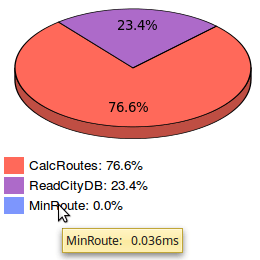
We have chosen the red color on purpose, as this response time is the determining factor for the overall response time. As shown in the image displayed on the right side, the computation of the shortest path takes about 76% of the total runtime.

Furthermore, we can see that the two subtasks ReadCityDB and CalcRoutes comprise almost all of the total runtime. The main program itself accounts for much less than 0.1% of the runtime: 0.036ms/731.9ms=0.004%!

Thus we will try to parallelize the computation of the shortest path in the next step!

In order to parallelize the algorithm we proceed as follows:

• As the algorithm we use is recursive we can rewrite the first recursion by using a loop:

  ForEach ListOfCities Do
    Remaining = ListOfCities
    Remaining.Remove(Current)
    Route.PushBack(Current)
    calcMinRoute(Remaining, Route, MinRoute)
  Done
  

• Now, we can parallelize this loop by corresponding OpenMP mechanisms

  #pragma omp parallel for
  ForEach ListOfCities Do
    Remaining = ListOfCities
    Remaining.Remove(Current)
    Route.PushBack(Current)
    calcMinRoute(Remaining, Route, MinRoute)
  Done
  

ARM 4.0 C++ instrumentation for parallel measurements

As we are parallelizing the computation of the shortest path, all measurements we are adding are sub-measurements belonging to the CalcRoute measurement. We thus need an ARM correlator for these types of measurement:

// get our parent ARM correlator
ArmCorrelator parent = calcRoute.getCorrelator();
// mark this correlator as asynchronous thus any sub-transaction is interpreted as asynchronous
parent.setAsynchronous(true);

We tag our ARM correlator as asynchronous, thus the analysis application will detect that those measurements are independent from other measurements. In this case, the SpeedUp factor can be computed (for the computation of T_p).

Here is our loop, parallelized by means of OpenMP and instrumented according to ARM 4.0:

// since we run in parallel we need to temporarily store each minimum route
std::vector<MinRoute> minRoutes(remaining.size());
#pragma omp parallel for
for(size_t i=0; i<remaining.size(); ++i)
{
   // create a partialRoute measurement for each loop entry
   ArmTransaction partialRoute(myARM::instance->myApp_, myARM::instance->partialRoutesDef_);
   // we automatically bind the measurement to the current thread
   partialRoute.setAutomaticBindThread(true);
   // start the partialRoute measurement with our parent correlator
   partialRoute.start(parent);
   // we need to create copies of our data to run independently
   std::vector<City*> ompRoute(route);
   std::vector<City*> stillRemaining(remaining);
   stillRemaining.erase(stillRemaining.begin()+i);
   ompRoute.push_back(remaining[i]);

   // we bind the MinRoute object for the i-th loop iteration to the function to call
   auto checkMinRoute = std::bind(&MinRoute::check, &minRoutes[i], std::placeholders::_1);
   // now build all routes and find the minimal route
   buildRoutes(stillRemaining, ompRoute, checkMinRoute);
   // now stop our partialRoute measurement
   partialRoute.stop(ArmConstants::STATUS_GOOD);
}

Recording and analysing parallel measurements

Now, we can start our freshly parallelized program ompRoute:

./ompRoute Berlin Hamburg München Köln "Frankfurt am Main" Stuttgart Dortmund Düsseldorf "Essen, Ruhr" Bremen

As expected, we get the same results:

route: |-- Berlin -[-sr255.292km]--> Hamburg --[95.2193km]--> Bremen --[196.644km]--> Dortmund --[33.239km]--> Essen, Ruhr --[30.189km]--> Düsseldorf --[33.377km]--> Köln --[152.598km]--> Frankfurt am Main --[152.705km]--> Stuttgart --[190.955km]--> München--| total distance is 1140.22km.

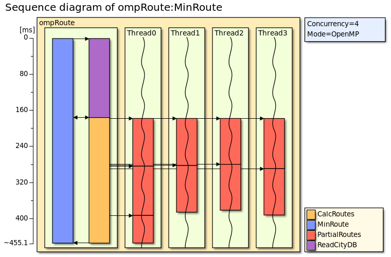
If running the program without explicitly specifying the number of threads to use (command line option -t num), the program will use as many threads as the number of CPU cores available. In our example, num=4.

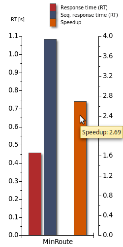
As you can see in the legend in the sequence diagram, the blue bar shows a response time of about 455ms for the entire calculation of the shortest path. Thus we have reduced the total response time by over 270ms! The purple bar shows the response time (about 175ms) for reading in the database of cities, the red bars show the response times for the corresponding partial paths. The orange bar shows the computation of the shortest path itself (about 279ms).

The Speedup diagram on the right side shows by how much we were able to speed up our algorithm by parallelizing:

• The first bar depicts the actual measured response time (wrt. the left Y axis)
• The second bar shows the response time as it would have been computed if all comprising parts would have been executed sequentially (wrt. to the left Y axis) - this is the so-called sequential response time
• The third bar shows the speedup factor (wrt. the right Y axis)

Please note that the sequential response time is about the same time that a single processor core would have been occupied for all computations. You could contrast this response time with the output of the Unix time command (user).

The parallelized version has spent about 250ms more CPU time than the sequential version.